Understanding Positional Encoding in Transformers

What is positional encoding?

As I’ve explained in “Introduction to Attention Mechanism”, attention doesn’t care about the position of the inputs. To fix that problem we have to introduce something called Positional Encoding. This encoding is covered in the original “Attention Is All You Need” paper and it’s added to every input (not concatenated but added).

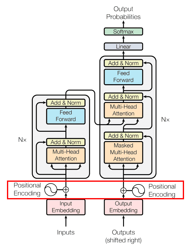
The paper only considered fixed (non-trainable) positional encoding and that’s what I’m going to explain. Right now encodings are trained along with the model but that requires another article. To calculate the value of positional encoding we have to go to section 3.5 in the paper. Authors are using sin and cos functions to calculate a value for every input vector.

$$PE_{(pos,2i)} = sin(\frac{pos}{10000^{2i/d_{\text{model}}}}) \newline \text{ } \newline PE_{(pos,2i+1)} = cos(\frac{pos}{10000^{2i/d_{\text{model}}}})$$

As you can see these values depend on $d_{model}$ (input dimension) and $i$ (index of the position vector). Original paper operates on 512 dimensional vectors but for simplicity I’m going to use $d_{model} = 50$ or $d_{model} = 20$. The authors also attached the comment about why they had chosen this kind of function:

We chose this function because we hypothesized it would allow the model to easily learn to attend by relative positions, since for any fixed offset $k$, $PE_{pos+k}$ can be represented as a linear function of $PE_{pos}$.

Positional encoding visualization

pos0

0

pos1

1

pos2

2

pos3

3

PrevNext

Values

We calculate the value for each index using the formula for a given index. It’s worth noticing that $2i$ value in $cos$ function is an even number so to calculate values for 0th and 1st indexes we’re going to use $sin(\frac{pos}{10000^{0/50}}) = sin(pos)$ and $cos(\frac{pos}{10000^{0/50}}) = cos(pos)$. That’s why values for 0th and 1st indexes are only dependent on the value of $pos$ instead of both $pos$ and $d_{model}$. This changes from the 2nd index onward because the dividend is no longer equal to 0, so the whole divisor is larger than 1 $(10000^{2i/50})$.

Dimension dependency

If you switch to the second step, then you can compare how the $PE$ value changes depend on $d_{model}$.

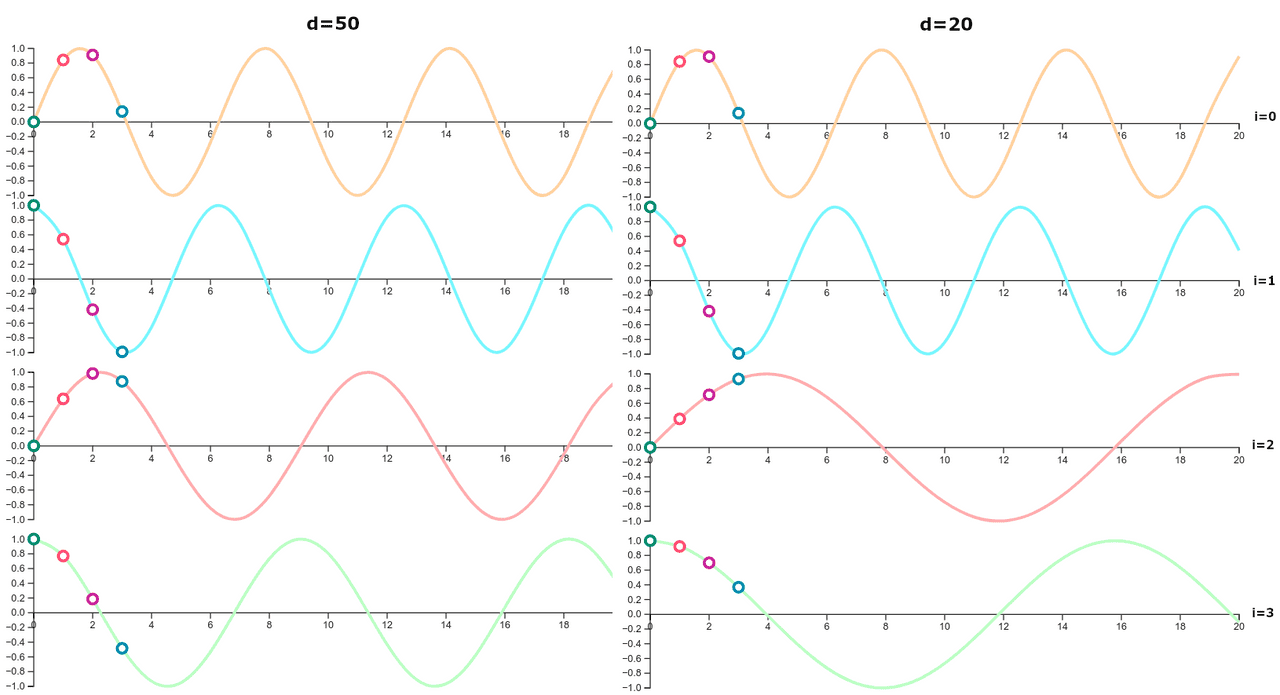
The period of the first two indexes is not changing with the change of $d_{model}$, but the period of further indexes (2nd and greater) widens with the decrease of $d_{model}$. This might be obvious, but it’s still good to see the difference.

Function periods

When we plot $PE$ values for the first 20 $pos$ vectors we get a result like that:

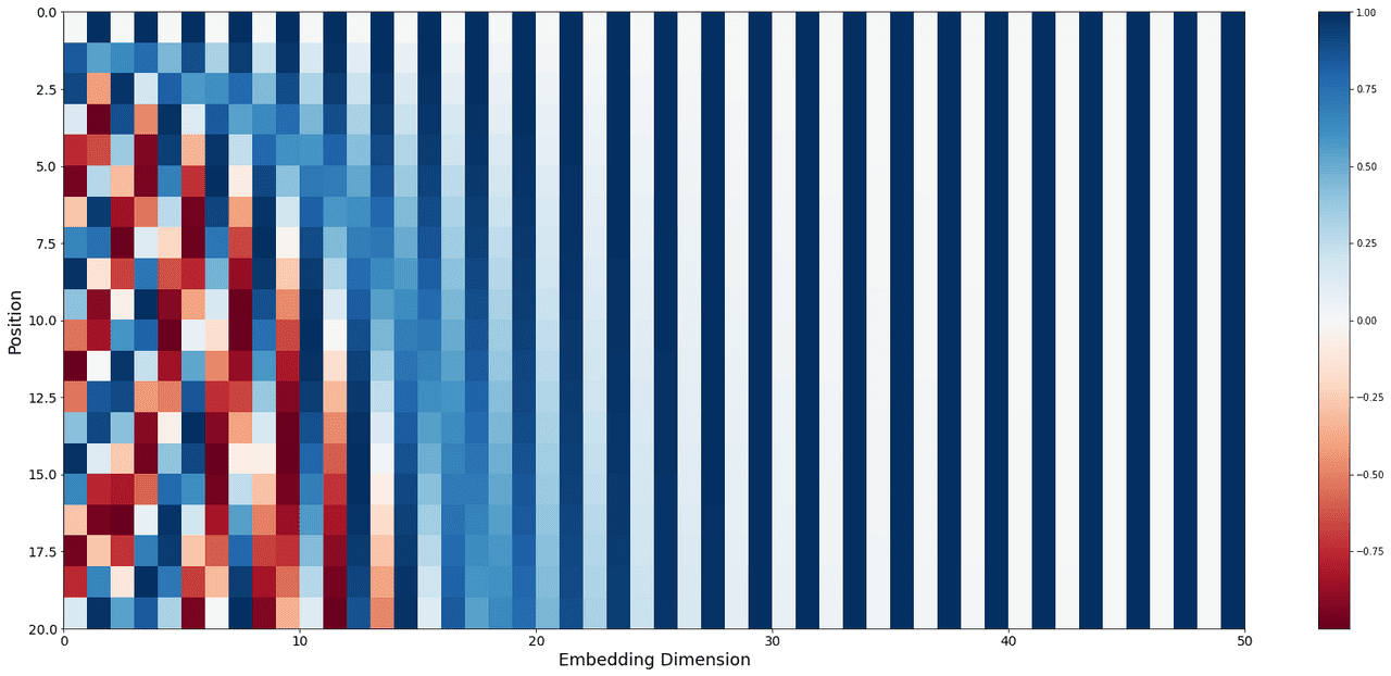
This plot is generated from one of Tensorflow’s Tutorials and you can run it with the help of Google Colab directly from their website. As you can see, lower dimensions of the position vector have a very short wavelength (distance between identical points). The wavelength of the function at $i = 6$ index has a wavelength around 19 ($2 * 10^{12/25}$).

We know that periods are increasing with the increase of $i$. When $i$ reaches the side of $d_{model}$, you need a lot of $pos$ vectors to cover the whole function period.

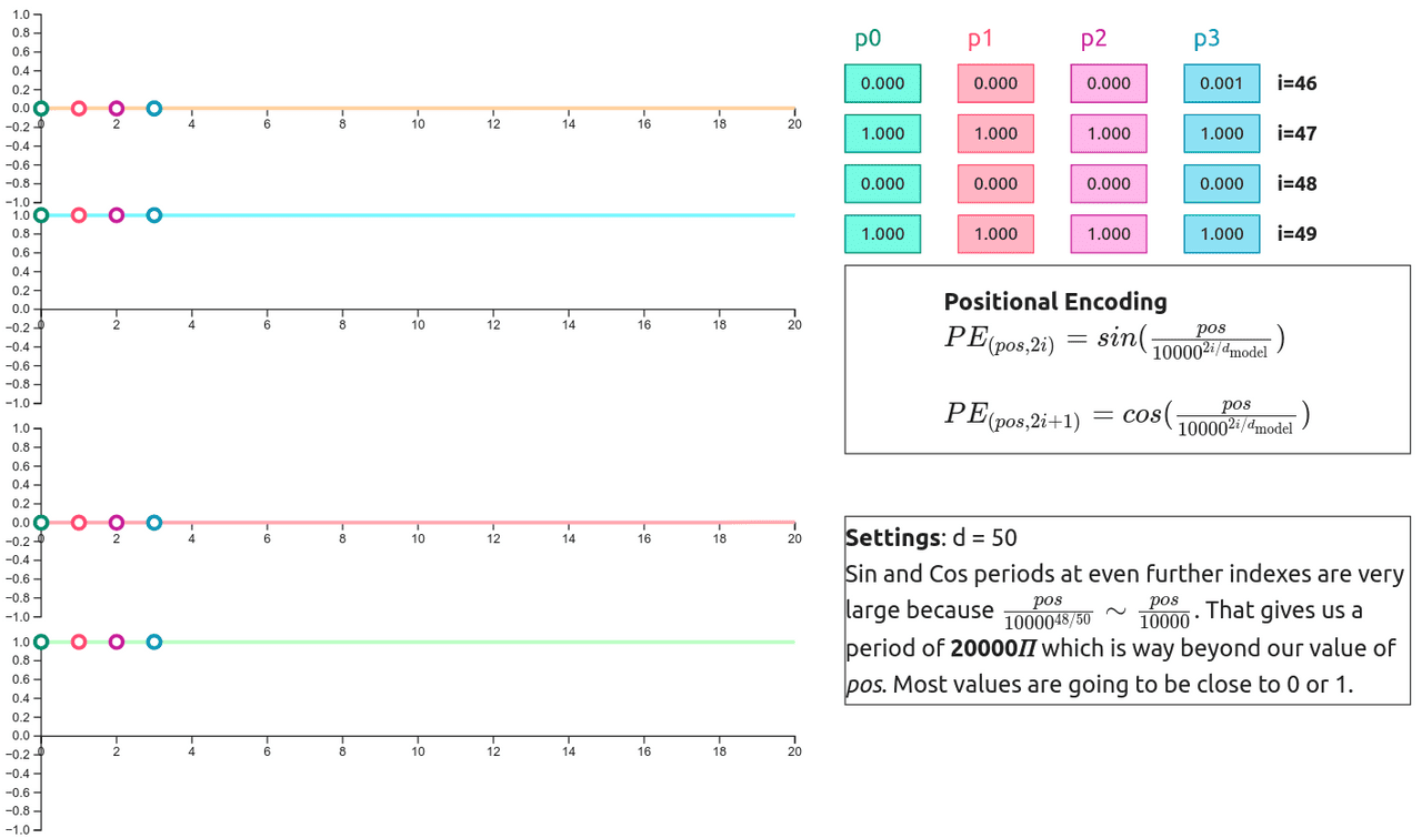
The values of the first 20 positions at the higher indexes are almost constant. You can see the same thing in Fig. 4 where the color of the columns 30-50 bearly change. To see that change we have to plot the values for tens of thousands of positions:

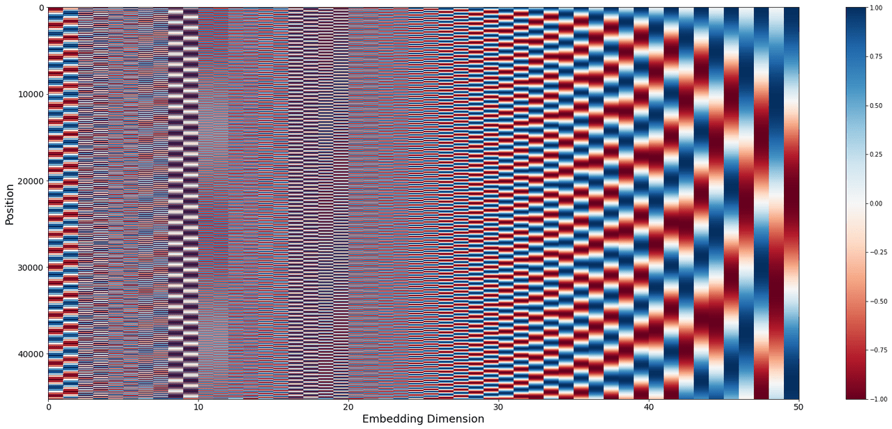
Warning This plot has a built-in illusion, it’s not actually an illusion but because it tries to print 40k+ values on 670px (height) it cannot show the correct value of anything with a wavelength smaller than 1px. That’s why anything prior to column 24 is visually incorrect even if the right values were used to generate this plot.

Conclusions

Positional embeddings are there to give a transformer knowledge about the position of the input vectors. They are added (not concatenated) to corresponding input vectors. Encoding depends on three values:

• $pos$ - position of the vector
• $i$ - index within the vector
• $d_{model}$ - dimension of the input

Value is calculated alternately with the help of the periodic functions ($sin$ and $cos$) and the wavelength of those functions increases with higher dimensions of the input vector. Values for indexes closer to the top of the vector (lower indexes) are changing quickly when those further away require a lot of positions to change a value (large periods).

This is just one way of doing positional encoding. Current SOTA models have encoders trained along with the model instead of using predefined functions. The authors even mentioned that option in the paper but didn’t notice a difference in the results:

We also experimented with using learned positional embeddings instead, and found that the two versions produced nearly identical results (see Table 3 row (E)). We chose the sinusoidal version because it may allow the model to extrapolate to sequence lengths longer than the ones encountered during training.

References:

• Ashish Vaswani et al, “Attention Is All You Need”, NeurIPS 2017 https://arxiv.org/abs/1706.03762