Introduction to Attention Mechanism

The attention mechanism is one of the most important inventions in Machine Learning, at this moment (2021) it’s used to achieve impressive results in almost every field of ML, and today I want to explain where it came from and how it works.

Before even beginning to explain Attention we have to go back and see the problem which Attention was supposed to solve. Before 2015, there was an issue with RNN which was occurred when the input sequence was really long.

PrevNext

This solution works fine as long as the sentence is short. After the decoder is done with its job, we’re left with the context vector c and the initial decoder state $s_0$. Those two vectors have to “summarize” the whole input sequence because we’re going to feed them into the decoder part of our model. You can treat the context vector as something that transferring information between the encoded sequence and the decoded sequence.

For long sentences, like T=100, it is highly probable that our context vector c is not going to be able to hold all meaningful information from the encoded sequence. Consider this quote:

“In a way, AI is both closer and farther off than we imagine. AI is closer to being able to do more powerful things than most people expect — driving cars, curing diseases, discovering planets, understanding media. Those will each have a great impact on the world, but we’re still figuring out what real intelligence is.” - Mark Zuckerberg in “Building Jarvis”

It is a lot easier to compress the first sentence to the context vector than to do the same for a whole quote. We could create longer and longer context vectors but because RNNs are sequential that won’t scale up. That’s where the Attention Mechanism comes in.

The idea is to create a new context vector every timestep of the decoder which attends differently to the encoded sequence.

PrevNext

This time we’re computing an additional context vector on every step of the decoder. Let us go through one whole step to explain what is happening.

1. Compute alignment scores

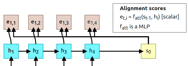
At $t=1$ we’re going to use $s_{t-1}$ decoder state to computer alignment scores. To compute the alignment score for every encoder state we’re using a function that is called alignment function but it’s just an MLP (MultiLayer Perceptron). Each alignment score can be treated as “how much $h_1$ is useful in predicting the output in the state $s_0$”. The alignment function outputs a scalar value which is a real number and we cannot use it just like that, we have to normalize those values using the softmax function.

2. Compute attention weights

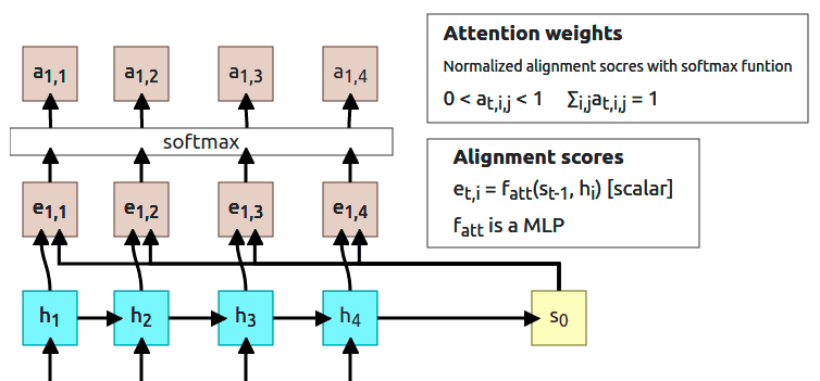
Output from the softmax function is normalized so all the numbers sum up to 1. Those outputs are called Attention weights and as the name says, they show the model “how much it should attend to corresponding hidden state”.

3. Compute context vector

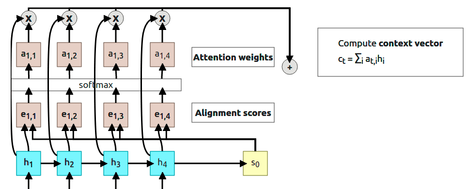
Now a lot of things happen (3 steps in the diagram above). First, we multiplied every attention weight by corresponding hidden state ($a_{1,1} \times h_{1,1}$, $a_{1,2} \times h_{1,2}$…). Then, all of the results are summed to use as a context vector $c_1$.

Note:
You’ve probably noticed that at this point “context vector” is actually a “context scalar” but this is just because we decided to have only 1D output (easier to show and understand for now). I’m going to switch to vectors when we get to abstracting attention to its own layer.

4. Compute the first output

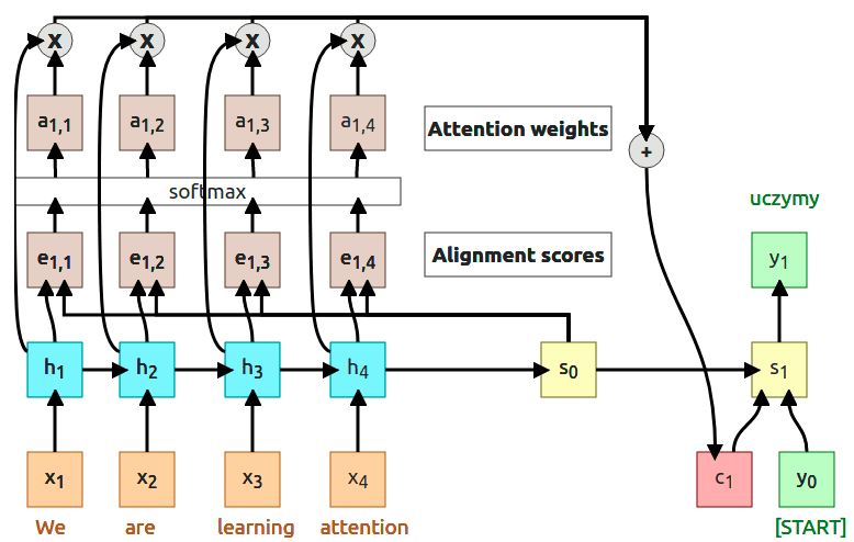
At the end of the first timestep, we can finally compute the first output from the decoder. That output is computed using context vector $c_1$, previous decoder’s state $s_0$, and start token $y_0$. Interesting thing is that in that whole process we don’t have to train $f_{att}$ as a separate model. The whole process is differentiable, so we can just backpropagate through the computational graph.

5. And repeat…

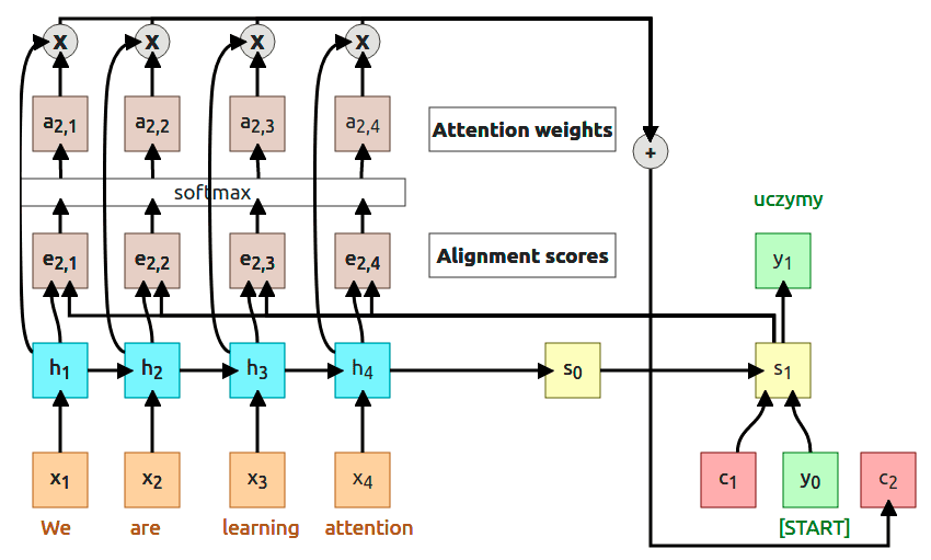
At the timestep $t=2$ only thing we have to do is to change the input to calculate the alignment scores from $s_0$ to $s_1$. Using the same process we compute new scores ($e_{2,1}$, $e_{2,1}$…) and attention weights ($a_{2,1}$, $a_{2,1}$…). Then multiply new attention weights and encoder’s hidden states to compute the new context vector $c_2$. At this point, the whole process just runs in the loop until the decoder produces [STOP] token (sometimes called [EOS] token, eng. End Of Sentence).

Attention weights visualization

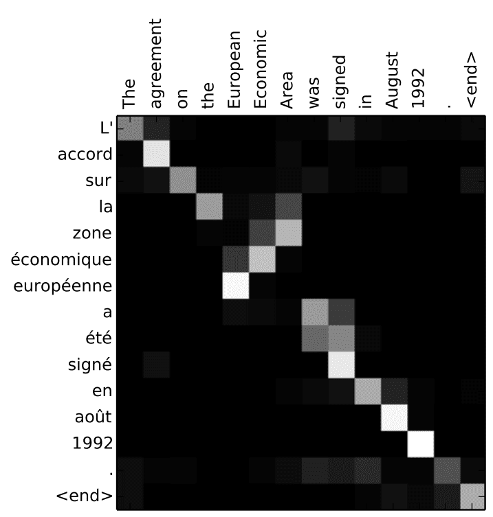
In the original paper, there is a simple visualization of the attention weights $a_{i,j}$ generated when translating the English sentence “The agreement on the European Economic Area was signed in August 1992.” into French “L’accord sur la zone économique européenne a été signé en août 1992.”. This visualization shows us a couple of interesting things.

The first thing is a diagonal pattern which tells us that model put more attention to corresponding French word from the same position. The second thing is more interesting and it is the phrase “European Economic Area” which in French has reverse order “la zone économique européenne”. We can see that when generating la token model puts more attention on the and Area, then when generating the zone token it attends to Area and Economic (ignoring European). Another interesting observation is “a été signé” where when generating a and été tokens, the model attends to both was and signed (it makes sense in French because we need to know an exact variation of the word étre).

This heatmap is important because we didn’t tell the model which words it should attend to, it learned this by itself. Additionally, we’ve got a kind of interpretability of the model’s decision.

Attention doesn’t know that input is a sequence

You probably started to worry about what happened with my information from the last step:

“We’re not using the fact that h vector is an ordered sequence. It is used as unordered set instead. To solve this we have to add a positional encoding to each element”

I’ve written a piece on positional encoding as a separate article because there is too much information to squeeze into this one. If you’re interested please check Understanding Positional Encoding in Transformers.

This is still a thing but instead of solving that problem, make use of it to abstract attention mechanism and use it for something different than a sequence of text. What about describing images with attention? There is a paper from the same year called “Show, Attend, and Tell: Neural Image Caption Generation with Visual Attention” that uses attention on CNN’s embedding to generate image captioning with the help of an RNN decoder.

PrevNext

In this paper, the authors are proposing a solution based on convolutional feature extraction instead of the standard RNN encoder network. We’re using those features from CNN to compute state and then to compute alignment scores for every timestep of the RNN decoder. As in the previous example, I’m going to walk you through the whole process, but you probably are able to understand it base on the interactive diagram above :)

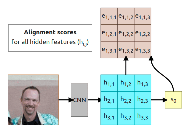
We’re assuming that CNN is already trained and produces our 3x3 grid. We’re going to use that initial grid to predict the initial hidden state $s_0$ (sometimes it could be randomly generated or even set to 0). Now we have to pass the same grid and $s_0$ to the alignment function to calculate corresponding alignment score for each value of the grid $e_{t,i,j} = f_{att}(s_{t-1}, h_{i,j})$. That gives us alignment scores for t=1 timestep. As in the previous example, each alignment score is a scalar which tells us “how important is given feature in the current timestep”.

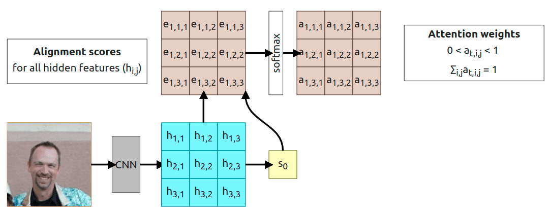
With alignment scores calculated we need to apply softmax to normalize scores to some probability distribution that sums to one.

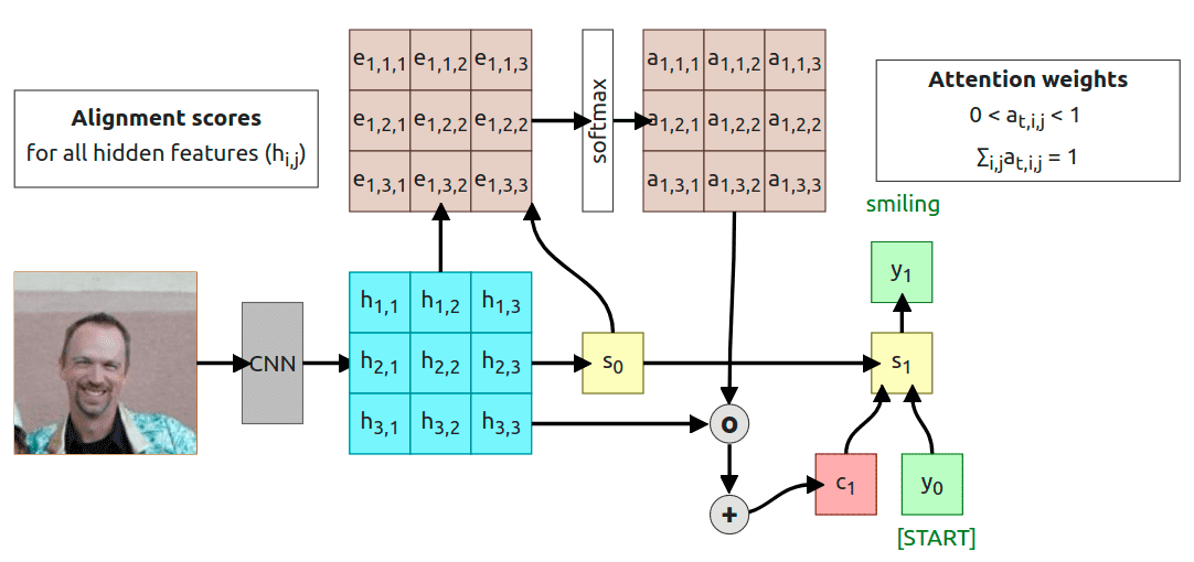
Now all we have to do is to compute Hadamard product (element-wise multiplication, $h_{i,j} \times a_{t,i,j}$ …) and sum everything to get a context vector $c_1$. The rest works exactly like in the previous example so we use context vector $c_1$, start token $y_0$, and initial decoder state $s_0$ and pass it through $g_U$ function to calculate $s_1$ state and achieve some output token $y_1$.

Note
The sum is not required at this point, I’m just doing it to have the same shape of the context vector as in the previous example. We could easily use a 3x3 matrix as an input to the $g_U$ function.

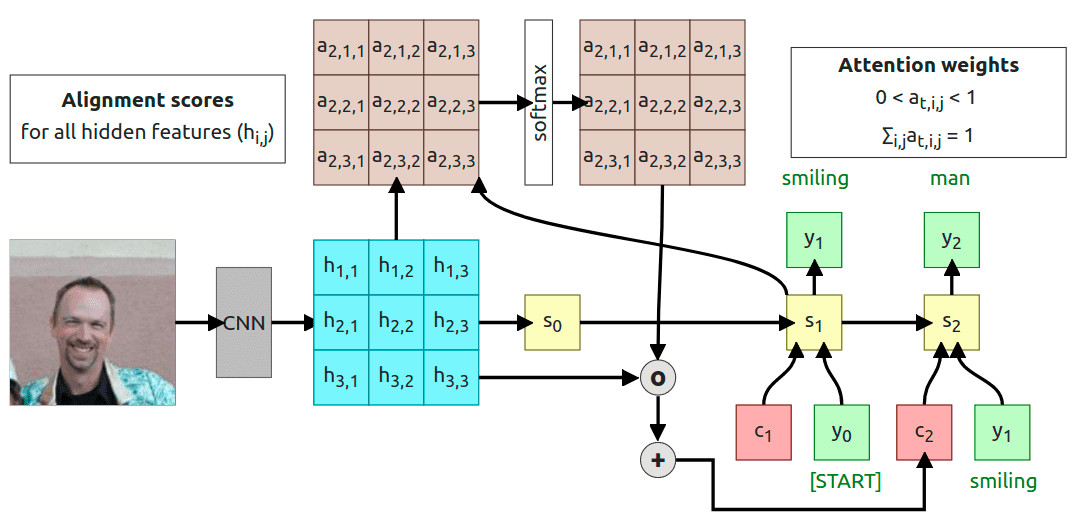
The same as before, we’re using newly generated $s_1$ state to compute new alignment scores $e_{2,i,j}$, which then are normalized with softmax and computed into context vector $c_2$. The process stops when the decoder produces [STOP] token as an output.

Visualization of the attention weights

The same as in sequence to sequence translation we are able to visualize attention weights in this case. I’m going to use one of the examples provided by the authors.

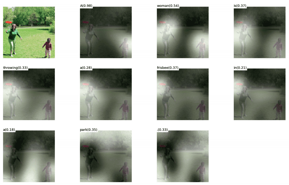
As you can see this is not an ideal solution for explaining a model but still could give you a kind of intuition about what is happening. Especially when we look at the tokens like frisbee or park when the model attends to those exact objects. In the case of the token woman, both people on the image save similar attention weights but that’s still ok because the model could decide which one is the subject and how to name that person.

There is one more type of attention called hard attention where instead of using the softmax function, we’re selecting a feature with the highest alignment score and using that feature’s value as a context. It requires some changes in the training process which I’m not going to discuss right now. Here is an example of hard attention.

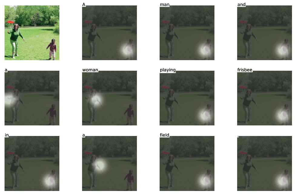
As you can see, the caption has changed. Now it’s saying “A man and a woman playing frisbee in a field.” instead “A woman is throwing a frisbee in a park.”. Attention regions are not fully related to the generated token (as in soft attention), when generating token frisbee model attends to the child.

Let’s abstract the Attention

Now, when you know what the Attention is, we can start working on abstracting the idea to create the so-called “Attention Layer”. First, let’s sum up what we have right now:

• Input vectors: X (shape $N_X \times D_X$)
• Query vector: q (shape $D_Q$), this is our previous hidden state, but I’ve changed the color to purpule to match the work from “The Illustrated Transformer”
• Similarity function: $f_{att}$
• Similarities: e, $e_i = f_{att}(\textcolor{mediumpurple}{q}, \textcolor{limegreen}{X_i})$
• Attention weights: $a = \text{softmax}(e)$ (shape $N_X$)
• Output: $y = \sum_i(a_i,\textcolor{limegreen}{X_i})$

Currently, our similarity function is $f_{att}$ which was correct, base on early attention papers but for the generalization, we can change it to be a dot product between q and X vectors. This is just a lot more efficient to calculate dot product, but it creates one product with the end results. As you remember, when calculating dot product of two vectors the results look like $\vec{a} \cdot \vec{b} = |\vec{a}| * |\vec{b}| * cos(\theta)$. This might cause a problem when the dimension of the vector is large. Why is it a problem? Look at the next step and the softmax function. It is a great function but can cause a vanishing gradient problem when the value of an element is really large and our value magnitude increases with the increase of the input dimension. That’s why you’re not using just a dot product, but a scaled dot product, that way our new $e_i$ formula looks like $e_i = \textcolor{mediumpurple}{q} \cdot \textcolor{limegreen}{X_i} / \sqrt{D_Q}$.

If you’re a having problem understanding why dot product creates a large number with high dimensional vectors please check 3Blue1Brown’s Youtube video on the subject

Additionally, we want to be able to use more than one query vector q. It was great to have a single query vector for each timestamp of the decoder but it can be a lot simpler when we use all of them at the same time, so we change our vector to vectors Q (Shape $N_Q \times D_Q$). This also affects the output shapes of the similarities scores and the attention:

• Input vectors: X (shape $N_X \times D_X$)
• Query vectors: Q (Shape $N_Q \times D_Q$)
• Similarity function: scaled dot product
• Similarities: $E = \textcolor{mediumpurple}{Q}\textcolor{limegreen}{X^T}$ (shape $N_Q \times N_X$), $E_{i,j} = \textcolor{mediumpurple}{Q_i} \cdot \textcolor{limegreen}{X_j} / \sqrt{D_Q}$
• Attention weights: $A = \text{softmax}(E, dim=1)$ (shape $N_Q \times N_X$)
• Output: $\textcolor{hotpink}{Y} = A\textcolor{limegreen}{X}$ (shape $N_Q \times D_X$) where $\textcolor{hotpink}{Y_i} = \sum_j(A_{i,j},\textcolor{limegreen}{X_j})$

You might wonder why softmax is calculated over dim=1? This is because we want to get a probability distribution for every query vector over input vectors. Another thing you should notice is that computation of the similarity scores simplified to just matrix multiplication.

The Layer

PrevNext

Now we’re getting into the juicy stuff. The first step on the diagram is a standard approach to attention. We have only our Query vectors and Input vectors. We’re using the input twice, once when computing Similarities and the second time when computing the Output vectors. We might want to use those vectors in a slightly different way and this is where the idea of Key and Value comes.

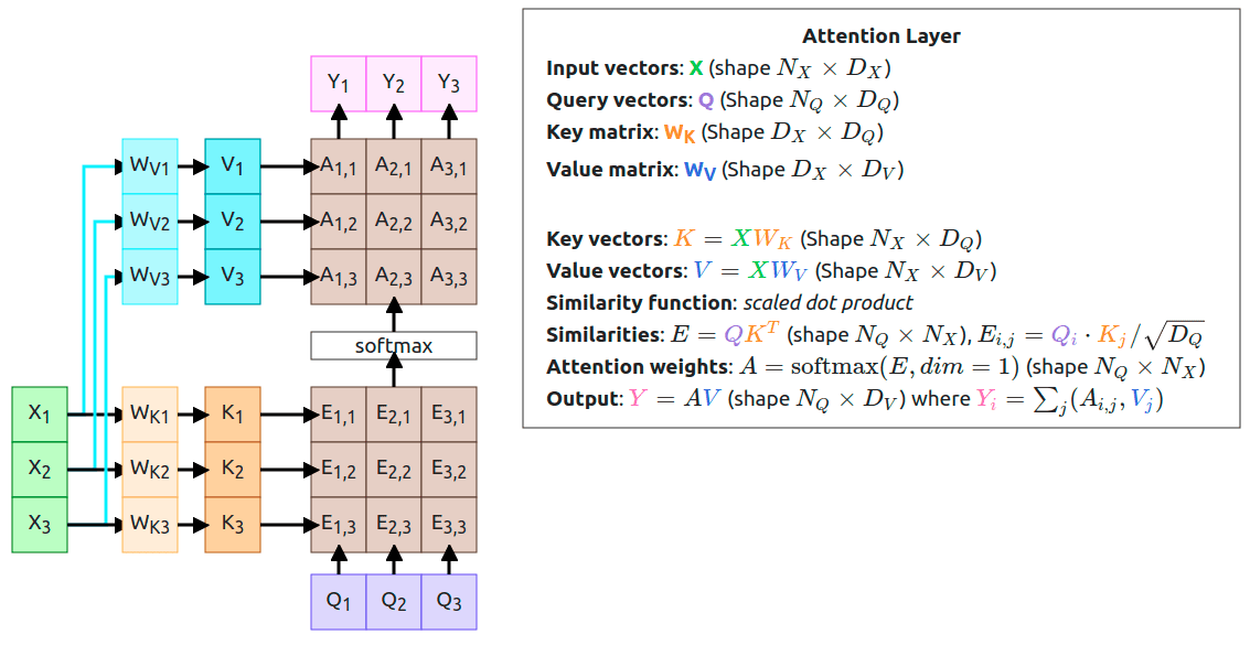
You might wonder what those vectors are and why are they important? I’ve found one intuition behind the general concept of query/value/key on the stackexchange:

The key/value/query concepts come from retrieval systems. For example, when you type a query to search for some video on Youtube, the search engine will map your query against a set of keys (video title, description, etc.) associated with candidate videos in the database, then present you the best matched videos (values).

If we look at that from a usability perspective, they allow the model to decide on how to use the input data. By creating trainable weights (W_K and W_V) we can adjust the input to fit different tasks.

Notice It just happens that all my vectors have the same length, exact shapes have to match (look at the shapes shown in the description), but they don’t have to be the same.

At this moment our Attention Layer is ready! Can we do even better? YES!!!

Self-Attention Layer

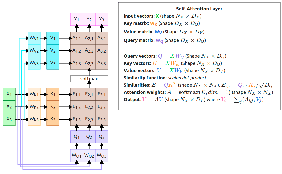
All this time, when using Attention Layer we were creating separate Query vectors and that has changed in the Self-Attention approach. This time we’re adding another weights matrix (W_Q) which is going to use in the computation of the new Query vectors. That way we’re enabling our model to learn a transformation of the Input vectors on its own.

What we have here is called Self-Attention Layer which is a general-purpose layer you can use in your model. It accepts Input vectors and outputs Output vectors. The whole layer is Permutation Equivariant ($f(s(x)) = s(f(x))$), that means when you permute the Input vectors output will be the same but permuted.

At last, I need to explain why I had changed the colors. The reason was to match the colors used in The Illustrated Transformer blog post.

Conclusions

From this point onwards we can use the Self-Attention Layer to create a Transformer but this article is too long already. You should have an intuition on how the attention mechanism works and why it works. I’m going to create another article on designing the Transformers and Multi-Headed Attention but for now please refer to The Illustrated Transformer.

Jay Alammar did a very good job explaining how transformers work and there is an additional example with vector computation. My post tries to explain how the idea of Attention and Self-Attention was created and because a lot of you come here after reading that blog post, I want you to feel familiar with the color schema.

I hope you’ve enjoyed the diagrams and if you have any questions please feel free to ask.

References:

• Sutskever et al, “Sequence to sequence learning with neural networks”, NeurIPS 2014 https://arxiv.org/abs/1409.3215
• Bahdanau et al, “Neural machine translation by jointly learning to align and translate”, ICLR 2015 https://arxiv.org/abs/1409.0473
• Xu et al, “Show, Attend, and Tell: Neural Image Caption Generation with Visual Attention”, ICML 2015 https://arxiv.org/abs/1502.03044
• Ashish Vaswani et al, “Attention Is All You Need”, NeurIPS 2017 https://arxiv.org/abs/1706.03762
• Jay Alammar, “The Illustrated Transformer”, 2018 http://jalammar.github.io/illustrated-transformer/
• 3Blue1Brown, “Dot products and duality | EoLA #9”, 2016 Youtube LyGKycYT2v0
• University of Michigan, “Deep Learning for Computer Vision”, 2019 Lectures